Part I: Representing M-ary Digital Modulation as Constellation Points
In M-ary digital modulation, we transmit one of \(M\) possible signals, \(s_1(t),s_2(t),\cdots,s_M(t)\), during each symbol interval of duration \(T\). Typically, \(M\) equals \(2^m\), where \(m\) is the number of bits per symbol. This makes the symbol duration \(T = m\cdot T_b\), where \(T_b\) is the bit duration.
M-ary modulation schemes are preferred over binary modulation schemes for transmitting digital data over bandpass channels when the requirement is to conserve bandwidth at the expense of both increased power and increased system complexity.
Bandwidth Conservation Capability of M-ary Modulation Schemes
Consider the transmission of information consisting of a binary sequence with a bit duration \(T_b\).
-
If we transmit information using binary phase shift keying (BPSK), the required channel bandwidth becomes proportional with \(1/T_b\).
-
If we take blocks of \(m\) bits to produce a symbol e.g. \(M\)-PSK with \(M=2^m\) and symbol duration \(T = m\cdot T_b\), then required channel bandwidth becomes proportional with \(1/(m\cdot T_b)\), which shows that the \(M\)-PSK reduces the required channel bandwidth by the factor of \(m = \log_2(M)\) over BPSK.
Mapping of Digitally Modulated Waveforms Onto Constellations of Signal Points
Starting with \(M\)-ary PSK due to its simplicity, the available phase \(2\pi\) radians are portioned equally and in a discrete way among \(M\) transmitted signals as follows:
\[s_i(t) = \sqrt{\frac{2E}{T}}\cos\left(2\pi f_c t + \frac{2\pi}{M}(i-1)\right)\]where \(i=1,\cdots,M\) and \(0 \leq t \leq T\). The parameter \(E\) is the signal energy per symbol and \(f_c\) is the carrier frequency.
The idea of signal-space diagrams has profound importance in statistical information theory since it provides a mathematical basis for the geometrical representation of energy signals, exemplified by digitally modulated waveforms. For a specific method of digital modulation, the geometric representation appears as constellation points in the signal space diagram, which is unique to that method. For instance, BPSK shows how two waveforms \(s_1(t)\) and \(s_2(t)\) representing the binary symbols \(1\) and \(0\) respectively, are mapped onto the transmitted signal points as follows:
\[\begin{aligned} s_1(t) &= \sqrt{\frac{2E_b}{T_b}}\cos(2\pi f_c t), ~~~\quad\quad \text{for bit 1} \\ s_2(t) &= \sqrt{\frac{2E_b}{T_b}}\cos(2\pi f_c t + \pi), \quad \text{for bit 0} \end{aligned}\]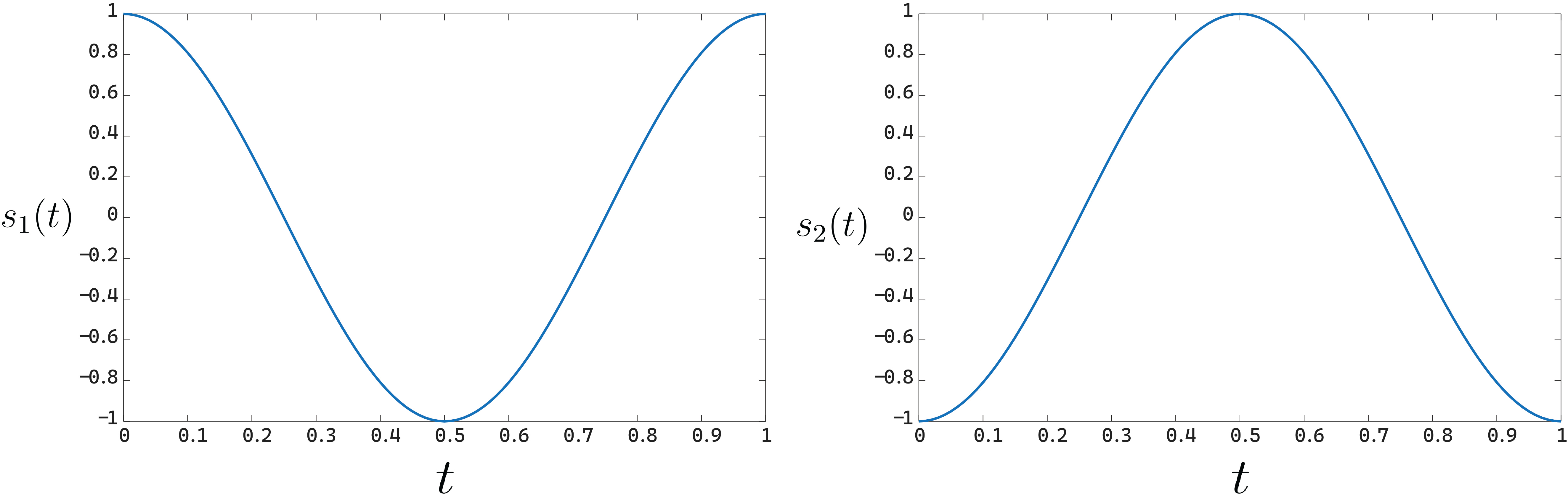
How is the mapping accomplished?
The answer lies within the concept of the correlator. The definition of the modulated waves for the BPSK modulation is given above. The signal-space representation of BPSK modulation involves a single basis function:
\[\phi_1(t) \sqrt{\frac{2}{T_b}}\cos(2\pi f_c t)\]The two signaling waveforms \(s_1(t)\) and \(s_2(t)\) are correlated with the basis function \(\phi_1(t)\), over the time interval \(0\leq t \leq T_b\). This is the same problem as designing a coherent BPSK receiver that can extract the information content from the transmitted signal,
-
We can extract the point \(\mathbf{s}_1\) by using, \(\mathbf{s}_1 = \int_{0}^{T_b}\phi_1(t)s_1(t)\text{d}t\).
-
Similarly, we can extract the point \(\mathbf{s}_2\) by using, \(\mathbf{s}_2 = \int_{0}^{T_b}\phi_1(t)s_2(t)\text{d}t\).
1) Let’s calculate the integral \(\mathbf{s}_1 = \int_{0}^{T_b}\phi_1(t)s_1(t)\text{d}t\),
\[\begin{aligned} \mathbf{s}_1 &= \int_{0}^{T_b} \left( \sqrt{\frac{2}{T_b}}\cos(2\pi f_c t) \right) \left( \sqrt\frac{2E_b}{T_b}\cos(2\pi f_c t) \right) \text{d}t \\ &= \int_{0}^{T_b}\frac{2\sqrt{E_b}}{T_b}\cos^2(2\pi f_c t) \end{aligned}\]Using the trigonometric identity:
\[\cos^2(\theta) = \frac{1 + \cos(2\theta)}{2}\]The integral evaluates to:
\[\begin{aligned} &\int_{0}^{T_b}\frac{2\sqrt{E_b}}{T_b}\cos^2(2\pi f_c t) \\ &= \int_{0}^{T_b}\frac{2\sqrt{E_b}}{T_b}\left( \frac{1 + \cos(4\pi f_c t)}{2} \right)\text{d}t \\ &= \frac{\sqrt{E_b}}{T_b}\int_{0}^{T_b} \text{d}t + \frac{\sqrt{E_b}}{T_b}\int_{0}^{T_b}\cos(4\pi f_c t) \text{d}t\end{aligned}\]Since \(\int_{0}^{T_b}\cos(4\pi f_c t) \text{d}t = 0\) (the area under the cosine curve for a full period), we get:
\[\mathbf{s}_1 = \frac{\sqrt{E_b}}{T_b}\int_{0}^{T_b} \text{d}t = \frac{\sqrt{E_b}}{T_b}\cdot T_b = \sqrt{E_b}\]2) Similarly for point \(\mathbf{s}_2\):
\[\begin{aligned} \mathbf{s}_2 &= \left( \sqrt{\frac{2}{T_b}}\cos(2\pi f_c t) \right) \left( \sqrt{\frac{2E_b}{T_b}}\cos(2\pi f_c t + \pi) \right)\text{d}t \\ &= \int_{0}^{T_b} \frac{2\sqrt{E_b}}{T_b}\cos(2\pi f_c t) \cos(2\pi f_c t + \pi) \text{d}t \end{aligned}\]Another well-known trigonometric expression is:
\[\begin{aligned} \cos(\theta + \gamma) &= \cos(\theta) \cos(\gamma) - \sin(\theta)\sin(\gamma) \\ \cos(\theta - \gamma) &= \cos(\theta) \cos(\gamma) + \sin(\theta)\sin(\gamma) \end{aligned}\]Therefore:
\[\cos(\theta)\cos(\gamma) = \frac{\cos(\theta+\gamma)+\cos(\theta-\gamma)}{2}\]Using this to evaluate the integral:
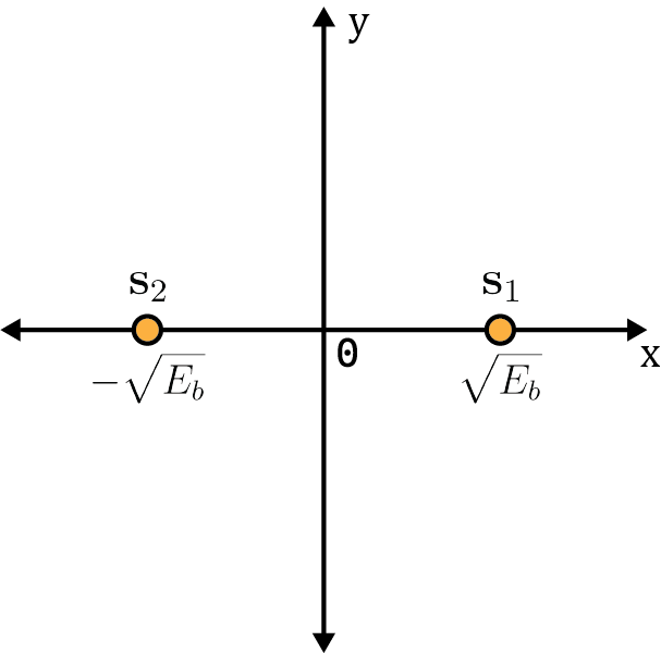
\[\begin{aligned} \mathbf{s}_2 &= \int_{0}^{T_b} \frac{2\sqrt{E_b}}{T_b}\cos(2\pi f_c t) \cos(2\pi f_c t + \pi) \text{d}t \\ &= \int_{0}^{T_b} \frac{2\sqrt{E_b}}{T_b} \left( \frac{\cos(4\pi f_c t + \pi) + \cos(-\pi)}{2}\right) \text{d}t \\ &= \frac{\sqrt{E_b}}{T_b}\int_{0}^{T_b}\cos(4\pi f_c t + \pi) \text{d}t - \frac{\sqrt{E_b}}{T_b}\int_{0}^{T_b} \text{d}t = -\sqrt{E_b} \end{aligned}\]The points \(\mathbf{s}_1\) and \(\mathbf{s}_2\) can be represented in a simple plot:
From PSK to QAM
References
[1] An Introduction to Digital and Analog Communications, Simon Haykin, 2nd Edition, 2001.
[2] Wireless Communications, Andrea Goldsmith, 2005.